In the series: Note 17.
Subject: The Grad and Div operators.
Date : 22 September, 2016Version: 0.4
By: Albert van der Sel
Doc. Number: Note 17.
For who: for beginners.
Remark: Please refresh the page to see any updates.
Status: Ready.
This note is especially for beginners.
Maybe you need to pick up "some" basic "mathematics" rather quickly.
So really..., my emphasis is on "rather quickly".
So, I am not sure of it, but I hope that this note can be of use.
Ofcourse, I hope you like my "style" and try the note anyway.
This note: Note 17: The Grad and Div operators.
Each note in this series, is build "on top" of the preceding ones.
Please be sure that you are on a "level" at least equivalent to the contents up to, and including, note 16.
Chapter 1. Some words on Rn -> Rm functions.
Linear algebra as a "tool":
Using "linear algebra", we have seen "linear transformations", defined on Rn -> Rm,which can be represented by a mxn matrix. This is a sort of "vectorial" approach.
Take notice of the fact how remarkably "general" such a theory as linear algebra actually is.
You might want to see math note 16, "Vector Calculus / Linear Algebra Part 2",
to see more on Matrix calculus and Operators.
This note will focus more on "analysis" instead of matrices/operators.
Analysis as a "tool":
On the other hand, we can use the approach from "calculus", or "analysis", which study functions in the broadest sense possible.So, in early notes in this series, we have seen quite a few y=f(x) functions (e.g. linear, quadratic, polynomials, goniometric functions like sin(x) etc...).
Usually, one starts with the study of functions of one variable like y=f(x).
However, in note 11, we started "scouting" functions of more variables, like z=f(x,y) and w=f(x,y.z).
Note that functions (or relations) of the form z=f(x,y), are relatively "easy" to interpret, since they often can be viewed
as "surfaces" in 3D space. If needed, take a look at note 11 again.
Here is a small sample of types of functions that can be studied using "classical" analysis:
-Scalar functions Rn -> R:
Indeed, analysis is a good theory to analyze Rn -> R functions. Yes, please be aware of the fact that a functionlike z = f(x,y) = x2 + y2 maps points (x,y) to the value "z", and thus is a R2 -> R function.
So, since the "endresults" of the functions are simply "scalars", mathematicians call them scalar functions.
As another example of a scalar function, this time from R3 -> R, take a look at:
w = φ(x,y,z) = 3x2y - y3z
For each point (x,y,z), it is mapped to a scalar "w".
-vector valued functions R -> Rn:
Analysis great for studing vector valued functions too. Here, that means that a single variable (like "x", or "t") is mapped to a vector.Take a look at these examples:
| F(t) = |
┌ sin(t) ┐ └ cos(t) ┘ |
Here real values "t" are mapped to 2 dimensional vectors.
Here is another example of a vector valued function:
| G(t) = |
┌ sin(t) ┐ │ 2t │ └ t ┘ |
Here real values "t" are mapped to 3 dimensional vectors.
A small warning here: Articles that study such sort of functions, often start with a "domain analysis". Since the components
of such function like G(t), are different functions by themselves, there might be ranges of "t", where such component fuction is not defined.
For example, a component function might be "ln(x)" or "1/t". So, for each component function, a mathematician must carefully
determine if possibly ranges of "t" are excluded.
-functions or mappings Rn -> Rm:
Analysis provide for methods to explore, and describe, functions that map Rn to Rm.Below is just an example to make the statement above rather plausible. So..., what would you think of the following mapping?
F((x, y, z)) = (2x 2y + z, 3x + y z, x + 5y, 6x 3y + 3z).
Or in column form:
| F((x, y, z)) = |
┌ 2x 2y + z ┐ │ 3x + y z │ │ x + 5y │ └ 6x 3y + 3z ┘ |
It's a mapping R3 -> R4. So, it's a mapping of 3 dimensional vectors, to 4 dimensional vectors. However, you notice that the
components in that mapping are by themselves, individual functions, like for example the third component "x + 5y".
By the way, the whole thing, that is "F" is a function too, and in this case, it can be proven that it is also a "linear map".
You can say that linear algebra, and analysis, are seperate sets of ideas and methods, but describe largely the same math and objecys.
But at the same time, they still have there own "specialties" (so to speak).
What is our main objective here?:
There exists certain "differentials" that provide extra information of the types of functions that we saw above.Those functions can for example be multi-variable scalar functions, like φ(x,y,z), or vector-valued functions.
Why would that be of importance?
The operations described below, are simply mathematically possible, and may provide extra insights of the functions themselves.
From a standpoint from physics, it's really great since the differentials give additional insights in physical processes.
Chapter 2. The gradient, or ∇ operator on a scalar function.
Suppose we have a scalar function φ(x,y,z).Then we know that, at regions where the function is "well-behaved" (like no gaps, no asymptotes etc..),
we can derive the partial derivatives like:
| ∂ φ(x,y,z) ---------- ∂ x |
, | ∂ φ(x,y,z) ---------- ∂ y |
, | ∂ φ(x,y,z) ---------- ∂ z |
If needed, take a look at note 11 again, where I introduced partial derivatives.
It's important to understand that for example the partial derivative on "x",
relates the rate of change of φ(x,y,z), compared to the the rate of change of "x".
Ofcourse a similar argument holds for the partial derivative on "y" and "z".
So, for each point (x,y,z), where φ(x,y,z) takes on a well-behaved value, we can calculate the partial derivatives.
Now, we may "make", which at first sight may seem, a remarkable construction.
If we construct a vector, with as components (or elements), the partial derivatives, then we have an
object that defines a "magnitude" and "direction", which characterizes the change of φ(x,y,z) with the change of space.
It's remarkable indeed. In a moment we dive a little more into how we must interpret this.
Recall that an often used notation voor the basis vectors in R3 is:
êx = (1,0,0) for the unit vector on the x-axis.
êy = (0,1,0) for the unit vector on the y-axis.
êz = (0,0,1) for the unit vector on the z-axis.
Our (new) vector is called the "Gradient" of φ(x,y,z) at point (x,y,z), and it is defined as:
| ∇ φ | = | ∂ φ(x,y,z) ---------- ∂ x |
êx | + | ∂ φ(x,y,z) ---------- ∂ y |
êy | + | ∂ φ(x,y,z) ---------- ∂ z |
êz | (equation 1) |
Or, written as a column vector:
| ∇ φ | = |
┌ ∂/∂x φ(x,y,z) ┐ │ ∂/∂y φ(x,y,z) │ └ ∂/∂z φ(x,y,z) ┘ |
(equation 2) |
The interpretation often found in physics is, that ∇ φ tells us how much φ vary (or changes) in the direct neighborhood
of some point (x, y, z).
Suppose that φ(x,y,z) is a measure of the strength of some "flow" (e.g. wind, water, or some other stream),
then ∇ φ gives us insight in the rate of changes of that flow (magnitude and direction) in space.
The example above, was about φ(x,y,z), thus a function of R3 -> R.
Nothing changes fundamentally, if φ was defined on Rn. Then, instead of (x, y, z), we would describe φ as φ(x1, x2, ..., xn), and the same
type of equations can be constructed as illustrated above.
Note that from equation 2, we can also say that we have a "grad operator", ∇, written as:
| ∇ | = |
┌ ∂/∂x ┐ │ ∂/∂y │ └ ∂/∂z ┘ |
(equation 3) |
Example:
Suppose, in a 3 dimensional Cartesian coordinate system, we have the scalar function:
φ(x,y,z) = 3x2 - 5y - sin(z)
Then the partial derivatives are: ∂/∂x φ(x,y,z) = 6x, ∂/∂y φ(x,y,z) = -5, ∂/∂x φ(x,y,z) = -cos(z).
Therefore:
∇ φ = (6x, -5, -cos(z))
And here ∇ φ is notated as a row vector.
Note that the rate of change of φ, now is known for every point (x, y, z) for which φ(x,y,z) is defined.
You can substitute any valid point (x,y,z), like e.g. (1,1,0) in ∇ φ, and you will get a specific vector.
This technique is used in many sciences, and also often implemented in computercode in order to graph flow-fields and the like.
Chapter 3. The Div operator on a vector-valued function.
In chapter 2, we saw how to construct a "vector" from using the "gradient" operator on a scalar function.-So, here, the "endresult" is a vector.
If we look at equation 3 again, we see that we can represent ∇ as a vector.
Now, if we have a vector-valued function "F", (thus a vector), then we can calculate the inner product
of ∇ with F. From note 12, we know that the inner product of two vectors, is a number (a scalar).
-So, here, the "endresult" is a scalar.
Ofcourse there is an "interpretation" (or explanation) of why we should do this type operation.
Let's first demonstrate the technique, and then discuss the interpretation (of why we would want to do this).
Suppose F is a vector valued function R3 -> R3
| F | = |
┌ Fx(x,y,z) ┐ │ Fy(x,y,z) │ └ Fz(x,y,z) ┘ |
Then we can calculate the "inner product" of ∇ and F in the usual way:
| ∇ · F | = |
┌ ∂/∂x ┐ │ ∂/∂y │ └ ∂/∂z ┘ |
· |
┌ Fx(x,y,z) ┐ │ Fy(x,y,z) │ └ Fz(x,y,z) ┘ |
| = | ∂/∂x Fx(x,y,z) + ∂/∂y Fy(x,y,z) + ∂/∂z Fz(x,y,z) | (equation 4) |
For a point (x,y,x), this operation returns a scalar. You may also compare equation 4 to equation 1.
Indeed, we do not see any basis vectors. Equation 4 is just a summation of numbers (for a certain point).
------------------------------------------------------------------
Maybe it can't hurt to place a small recap from note 12 here, on the inner product in R3:
Recall that (from note 12), that, using an orthonormal Cartesian basis in R3,
the inner product is calculated as follows:
| A = |
┌ a1 ┐ │ a2 │ └ a3 ┘ |
| B = |
┌ b1 ┐ │ b2 │ └ b3 ┘ |
Then the "inner product" (also called "dot product") is defined to be:
| A · B = |
a1b1+a2b2+a3b3 |
In many articles and textbooks, the inner product as in equation 4, is also often denoted as Div F, thus:
Div F = ∇ · F
So, what is behind it? How can we interpret ∇ · F?Maybe the idea of "flux" can contribute to this.
The Flux Φ of a vector field.
Suppose we have some vectorfield in space, like an Electric Field, or a Magnetic field.
However, if you like something like the flow of wind (or water etc..), then that's is fine with me too.
Everything is ok, as long as you mentally can "imagine" a sort of vector field.
-Now, also imaging an open Surface like a square (or other figure).
Also imaging the field passing through that Surface. If the field is weak, we say that the "Flux" (Φ) through
the surface is low. But suppose that the field is very intense, then we say that Φ is high.
(1). If the field is perpendicular to the surface, Φ has it maximum value.
(2). If the field is parallel to the surface, Φ is "0".
(3). If there is an angle between the surface and the field, only the perpendicular component of the field contributes to the Φ.
So, Φ is a measure for the number (of intensity) of fieldlines passing through a surface.
If the field gets stronger, then Φ gets larger, and if the surface area "A" increases, then Φ increases too.
Figure 1. Some example of the flux through a surface
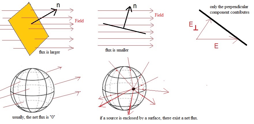
For a flat surface, and a uniform field F perpendicular to "A", then Φ = |F||A|.
If there is an angle α between the uniform field and the flat surface area, then Φ = |F||A| cos(α).
-Now imagine a closed surface, around a volume, like a sphere, or peach-like volume, or something like that.
If fieldlines pass through such a surface, you may wonder what the "total" flux is.
From a certain side, fieldlines enter the surface, but may exit that surface at the other side.
Makes it really sense to talk of a "net" flux?
-On thing is for sure: if the source of the field is "inside" the surface, and fieldlines only pour outwards
through the surface, then we absolutely have a netto flux through the surface. Also, suppose a "field sink" is inside,
then we may have only fieldlines enter the surface, and never come out. This yields a netto total flux too.
-For some Physical fields, it is true that for any closed surface, then the total flux through that closed surface is "0".
For example, for a magnetic field, Div B = 0.
Further analysis of equation 4.
Let's take a look at this part from equation 4:
∂/∂x Fx(x,y,z) + ∂/∂y Fy(x,y,z) + ∂/∂z Fz(x,y,z)
It represents the infinitsemal change of F in an infinitsemal small region.That statement cannot surprise you. Even with a function of one variable, y=f(x), we know that df(x)/dx represents the infinitsemal
change of "f" compared to the infinitsemal change of "x".
Let's now look at a very small volume, say a cube if you will, somewhere in the vectorfield, and see if we can determine
the flux through the tiny surface of that cube.
Say that the (extremely small) volume "η" can be characterized by "Δ x Δ y Δ z".
Figure 2. A very small volume, and the flux through the surface
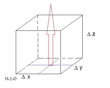
You do not need to remeber the following reasoning. Just read it, since it helps in understanding the meaning of ∇ · F.
We want to determine the difference in flux, through the lower z-plane of "η", and the upper z-plane of "η".
Then we will do the same for the y- and x-planes of the cube "η".
In first order approximation, the difference in the Fz component with respect to the
lower- and upper z-plane of "η", is:
∂/∂z Fz · Δ z
Fz will change extremely little in an infinitesemal distance dz, but over Δ z, we have the change in Fz
as described above.
Now, the difference in flux then would be "Surface * ∂/∂z Fz · Δ z" which then would yield:
Δ Φz = Δ x Δ y * ∂/∂z Fz · Δ z
since Δ x Δ y represents the surface of such a z-plane of "η"
Now, we can do the same thing for the differences of the y- and x-planes of our cube "η".
If we work that out, and add the other 2 results to our result found voor the z-planes, we have:
netto Flux =
(Δ x Δ y * ∂/∂z Fz · Δ z) +
(Δ y Δ z * ∂/∂x Fx · Δ x) +
(Δ x Δ z * ∂/∂y Fy · Δ y)
=
(Δ x Δ y Δ z * ∂/∂z Fz) +
(Δ y Δ z Δ x * ∂/∂x Fx) +
(Δ x Δ z Δ y * ∂/∂y Fy)
= (Δ x Δ y Δ z) (∂/∂x Fx + ∂/∂y Fy + (∂/∂z Fz)
-Note that the second "string" is ∇ · F (as we know from equation 4).
-Note that Δ x Δ y Δ z is the volume of our small cube "η".
Thus we have:netto Flux = (volume η) (∇ · F)
It's the same sort of equation as "a = b x c". We have a=0 if c=0, if b has a certain value, no matter how small.And if c=0, then a=0.
So, if we have a small volume, and some net flux is coming out (or in), then ∇ · F is not nul.
Also, if we have a small volume, no flux is coming out (or in), then ∇ · F is nul.
If there is a net flux, then something of a source that "diverges" or "generates" the field, must exist in the
immediate neighborhoud of the point (x, y, z).
That's why ∇ · F is also called Div F (divergence F).
For example, a stationary point charge sits in Δ x Δ y Δ z, which is responsible for an Electric field.
Then, ∇ · F will not be zero.
If that point charge is outside Δ x Δ y Δ z, then ∇ · F = 0.
Remarkably, the divergence of the Magnetic field (Div B) is nul. But a magnetic monopole has never been observed.
This is a classical approach, and physicists believe that true point-like particles are no reality.
However, for a classical vectorfield, the theory holds up.
Although the discussion above will not get the first prize, it hopefully gave an understanding of ∇ · F.
I originally planned to do "Curl F = ∇ x F" as well in this note, but a little more physics
needs to be introduced first (I think). So we will see that in the "Basic series on Physics".